Center for the Study of Complex Systems
Recent News
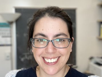
Catching up on the news : CSCS Director Marisa Eisenberg
In the fall of 2023 Professor Eisenberg became co-director of the MICOM CDC Center for Forecasting and Outbreak Analytics; and she continues to make news tracking COVID outbreaks with more reliable wastewater monitoring - as seen in NYT
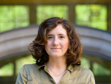
Professor Abigail Jacobs: prestigious fellowship and impactful article published.
Professor Jacobs was appointed to the inaugural co-hort of the Microsoft Research AI & Society Fellows; and is receiving press coverage for her preprint that uncovers that AI related to motion capture is being built on dated, flawed data..and cadavers?
WELCOME TO THE CENTER FOR THE STUDY OF COMPLEX SYSTEMS
The Center for the Study of Complex Systems (CSCS) is a broadly interdisciplinary program in the College of Literature, Science and the Arts (LSA) at the University of Michigan in Ann Arbor, Michigan. Our mission is to encourage and facilitate research and education in the general area of nonlinear, dynamical and adaptive systems.
CLICK TO WATCH THE COMPLEX SYSTEMS ANIMATED VIDEO EXPLAINER
"What IS Complex Systems"
Maybe you’ve seen the Center for the Study of Complex Systems at the University of Michgian and wondered ‘what ARE complex systems’? This animated video was prepared to provide a general explanation of the field of Complex Systems Science.
Oh, and we are a Center that is housed within the College of Literature, Science and the Arts, that offers a Minor and a Graduate Certificate.
We strive to support our students and faculty on the front lines of learning and research and to steward our planet, our community, our campus. To do this, the Center for the Study of Complex Systems needs your support.
The University of Michigan, named after Michigamaa (“Great Water” in Ojibwe), occupies the traditional territory stewarded by the Anishinaabe. This land was ceded through the Treaty of Fort Meigs by the Anishinaabeg—the Three Fires People—Ojibwe (Chippewa), Odawa (Ottawa) and Bodewadimi (Potawatomi). Through these words their current and ancestral ties to the land and to the University are acknowledged.